Quest 1 of 15
Python & Mathematics for Machine Learning
Build the mathematical intuition developers need: vectors and matrices (NumPy), derivatives and gradients, probability, and basic statistics — implemented in code before touching frameworks. Inspired by ML foundations curricula (linear algebra → calculus → probability), you will implement dot products, matrix multiply, and a simple gradient step by hand. For example, you will express a linear model as y = Wx + b and update weights one step with a computed gradient.
Start here
If you can write basic Python but the mathematics of machine learning feels abstract, start here. We will connect arrays, functions, derivatives, and probability to one concrete task: fitting a model that turns input features into useful predictions.
Big idea
Most supervised machine learning can be described as a loop: represent examples as numbers, use parameters to make predictions, measure prediction error with a loss function, and adjust the parameters to reduce that loss. Linear algebra makes this efficient across batches of data; calculus tells us how each parameter affects error; probability helps us describe uncertainty.
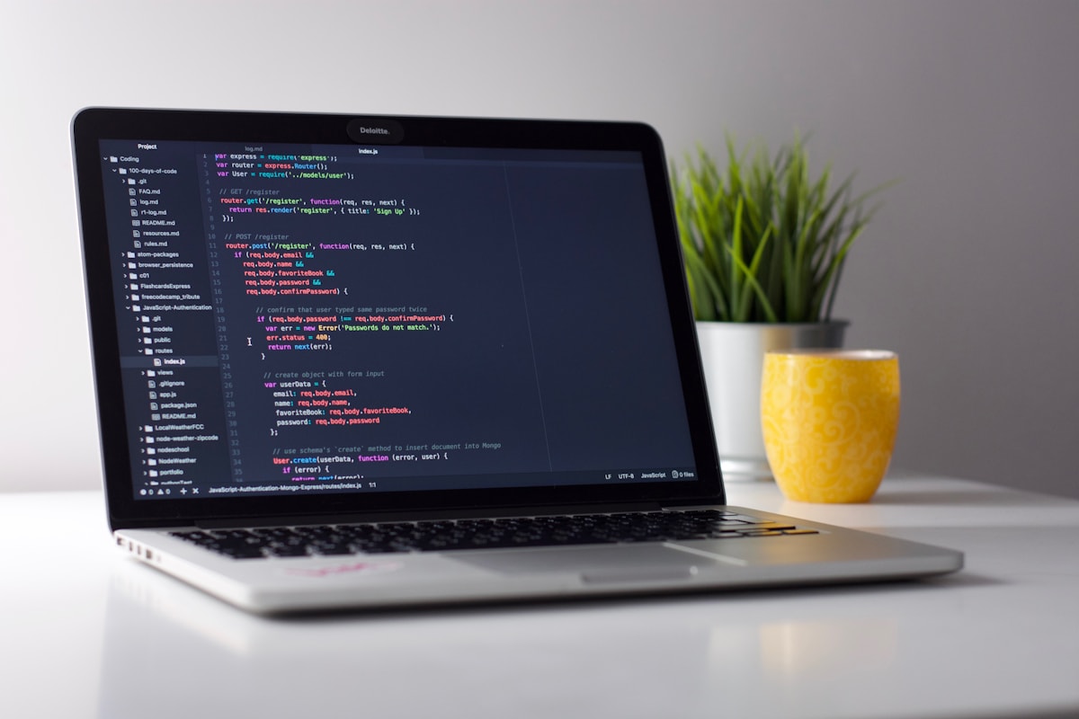
From data matrix to gradient step
Rows = samples, columns = features.
Learn one idea at a time
Read, explore, then mark each idea when you can explain it.
Idea 1 of 8
Represent a tabular dataset as a matrix X: each row is one example and each column is a measurable feature. In a house-price example, a row might contain floor area, bedroom count, and distance from the city centre. The target vector y stores the known sale price for each row. Printing shapes such as X.shape == (1000, 3) is a simple habit that prevents many bugs.
Choose a deep dive
Open the topics you want to explore. The detail stays folded until you need it.
Deep dive 1Worked example: one gradient-descent step
Suppose a one-feature model predicts delivery time from distance using prediction = distance × weight. With weight 2, a 10 km trip predicts 20 minutes, but the observed time is 30. The loss says the prediction is too low, and the gradient shows that increasing the weight would reduce error. The optimiser updates the weight slightly, then repeats across many trips. Real networks contain millions of parameters, but autograd performs this same chain of sensitivity calculations.
Deep dive 2Why dimensions matter
If X has shape (batch_size, features) and w has shape (features,), X @ w returns one prediction per row. If preprocessing unexpectedly adds or removes a column, matrix multiplication fails—or worse, reordered columns silently produce wrong predictions. Define feature schemas, assert shapes, and test preprocessing independently before blaming the model architecture.
Deep dive 3Shape errors are the #1 beginner bug
Print .shape after every matrix operation. Most PyTorch errors are (N, C, H, W) vs (N, H, W) confusion — fix shapes before tuning architecture.
Deep dive 4Probability powers loss functions
Cross-entropy connects predicted probabilities to true labels. Maximum likelihood estimation is the statistical story behind many ML loss functions.
Deep dive 5Worked example: linear regression from scratch in 20 lines
Generate synthetic data: X = np.random.rand(100, 1) * 10 and y = 3 * X + 4 + noise. Initialise w = 0, b = 0. Each epoch: compute predictions y_hat = X @ w + b, loss = ((y_hat - y) ** 2).mean(), then the gradients dw = 2 * (X * (y_hat - y)).mean() and db = 2 * (y_hat - y).mean(), and update w -= lr * dw; b -= lr * db. After a few hundred epochs with lr=0.01, w approaches 3 and b approaches 4. Now change lr to 1.0 and watch the loss oscillate and diverge; change it to 1e-5 and watch it crawl. You have now personally experienced the learning-rate trade-off that every deep-learning run in your career will repeat at scale.
Deep dive 6The chain rule is the whole trick
Backpropagation is the chain rule applied systematically. If loss depends on a prediction, the prediction on a weighted sum, and the sum on each weight, then the derivative of loss with respect to each weight is the product of the local derivatives along that path. A computation graph organises millions of such paths so each gradient is computed once, efficiently, in a backward sweep. When you later call loss.backward(), picture exactly this: local derivatives multiplying along paths from the loss back to every parameter. Frameworks automate the bookkeeping; the mathematics is one rule you already know from calculus.
Deep dive 7Math in code first
Implement one gradient step in NumPy before trusting autograd.
One-minute challenge
Connect this lesson to real life
Name one situation where this idea could help, and one thing a person should still check.
Explore a real-world example
Use the arrows to connect the idea to a visible situation.
Photo example
Example: shapes
Print .shape after every matrix op — it saves hours.

Key terms
Tap a term to flip and read the definition.
Optional further learningFree textbooks and trusted online resources
These sources informed the course structure. Use them to revisit a concept or study it in more depth.
Ready check
Tick each idea only when you could explain it without looking back.
Ready for practice? Complete the NumPy and gradient-descent labs before Module 2.
Extra context (audience, logistics, curriculum notes)
Built for: Software developers and technical learners with basic Python. Comfort with functions, loops, and installing packages required.
Formats: Coding labs · Math intuition exercises · Interactive quiz · Optional chat lab
Developer track Module 1 — math foundations for ML (NumPy, vectors, gradients, probability).
Next up
Ready for the next part?
When you've finished the reading, inline exercises, and knowledge check for this part, check the box to continue.